
The longevity of polymers in real-world use is a critical importance across industries, from medical devices and packaging to consumer products and infrastructure. While many polymers are engineered to withstand sunlight, heat, moisture, and chemical exposure, nearly everyone has seen a once-flexible product turn brittle, discolored, or cracked over time. Both raw materials (such as pellets or powders) and finished products can slowly degrade in storage or use, leading to cosmetic changes or even complete functional failure.
Because real-time testing of decades-long product lifespans is rarely practical, manufacturers rely on accelerated aging studies to estimate a polymer’s shelf life and in-use performance. These tests subject materials to elevated stress conditions that replicate the effects of long-term aging within a much shorter timeframe, providing scientifically grounded predictions of stability.
Accelerated Aging and the Arrhenius Equation
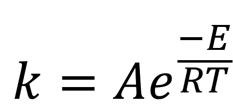
A common approach to accelerated aging is through heat, exploiting the known exponential relationship between temperature and reaction rates described in the Arrhenius equation, as shown in Equation 1, where k is the reaction rate, E is the activation energy for the reaction, T is the temperature of the storage environment, and R is the universal gas constant (8.314 JK-1mol-1). A is a prefactor term that is usually determined empirically.
Equation 1
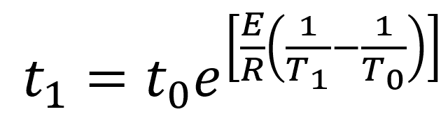
In an accelerated aging study, the researcher establishes a property that will be affected by aging and then sets a threshold limit on that property where the material or product no longer meets its specifications. Experiments can then be conducted at various temperatures over time to determine the time to failure at these temperatures. Equation 1 can be re-written in terms of time to failure t1 at the accelerated temperature T1 relative to the real time conditions (time to failure t0 at real-time temperature T0) as:
Equation 2
By determining reaction rate at two different temperatures, the A prefactor is not needed and the only unknown in these equations is the activation energy. This parameter is a function of the material and how it was processed and describes the minimum amount of energy required to initiate a chemical reaction. There are a few ways of experimentally determine the activation energy (or in some cases tabulated values can be used).
Determining Activation Energy
ASTM D3045 Approach
In one method, samples are aged at four or more temperatures for varying amounts of time, and the property of interest, such as tensile strength, is measured for each of these specimens over time (see Figure 1 and Figure 2).
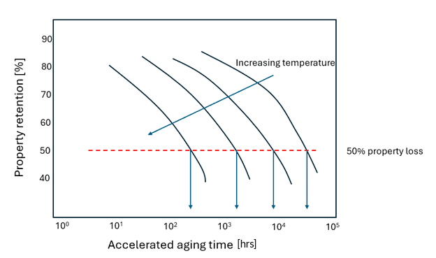
Figure 1: Property loss as a function of temperature following ASTM D3045 at four different temperatures. The related time to failure values are noted with the downward facing arrows, which are used in Figure 2.
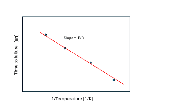
Figure 2: Determination of activation energy, E, from Figure 1.
A threshold property value is used to plot a time versus inverse temperature plot (Figure 2), the slope of which yields activation energy. This method is a reliable way of determining the activation energy, which can then be used for assessing property loss at different storage temperatures. The downside of this approach is that many experiments (and time) are required to build a dataset.
ASTM E1641 Approach
A quicker approach is to determine the activation energy through ASTM E1641, where a set of thermogravimetric analyses (using a Thermogravimetric Analyzer, or TGA) at different heating rates are used to monitor thermally-driven mass loss. In a simple system, the thermally-driven mass loss is an indication of the resistance of the material to thermal decomposition, and the heating rate provides the kinetic driver for the testing. By testing four samples at different heating rates and selecting a target mass loss (say 5%), a plot of log (heating rate) vs. (1/T), similar to Figure 2, will be generated, with the slope proportional to the activation energy. However, it should be noted that in our experience, the calculated activation energy of these two techniques is rarely identical.
Dynamic Rheology / Master-Curve Approach
There is a third common technique for polymers. The dynamic rheological properties of a polymer also generally obey the Arrhenius function and therefore building a so-called master-curve from a set of rheological experiments at different experiments. The shift factor used to create this master-curve is related to the activation energy of the polymer, providing another way to estimate this important parameter.
Simplifying with the Q10 Factor
Discussing aging rates in terms of activation energies can be unwieldly. As a result, researchers performing accelerated aging studies often refer to the Q10 value, which is the pre-factor that considers how much the reaction rate Rn with an increase of 10 ºC. The Q10 factor is simply written as:
Equation 3
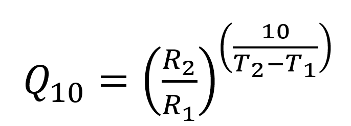
where R1 and R2 are the reaction rates at the respective temperatures. The Q10 can be determined from the activation energy through manipulation of Equation 2 and Equation 3. Knowing a Q10 value for your material or product, you can quickly see real time (RT) shelf-life equivalent values based on accelerated aging temperatures (A) by rearranging Equation 3 to get:
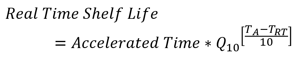
This process is captured in ASTM F1980. As an example, for a Q10 of 2.0, accelerated aging for 30 days at 50 ºC relative to real time storage conditions at 23 ºC would give a real time equivalence of 195 days. Often this value of Q10 is used as a default value, but selection of the accelerated aging temperatures, and calculation of an accurate Q10, requires detailed knowledge of the materials used.
Learn More in Our Accelerated Aging Webinar
To explore these concepts in more depth, including practical limitations and real-world examples, attend our webinar:
Age ISN’T Just A Number: Accelerated Aging Methods for Material and Product Characterization
Date: Wed, Jan 21, 2026
Time: 2:00 – 3:00 PM EST
In this presentation, we will discuss accelerated aging as a ubiquitous tool used to ensure shelf and in-use stability over long time periods. This powerful collection of techniques allows prediction of potential aging issues that would be time consuming and costly to identify in real time. However, accelerated aging has limitations, and data generated in an accelerated study must not be used blindly.
CPG Speakers
- Gavin Braithwaite, Chief Executive Officer
- Jaimee Robertson, Director of Consulting Services
- Kalpana Viswanathan, Polymer Chemist
The webinar will:
- Review aging mechanisms in polymers and the scientific assumptions that underpin accelerated aging.
- Discuss analytical techniques that can be used to screen material aging or infer acceleration factors, including their weaknesses.
- Present a case study comparing accelerated aging techniques to demonstrate the importance of careful experimental design when relying on accelerated methods to predict material performance.
Attendees will gain an understanding of the processes underpinning accelerated aging and the key considerations for applying these data to material and product decisions.
Secure your spot.
Partner with Cambridge Polymer Group
Selecting effective appropriate accelerated aging conditions requires a solid understanding of your product’s material composition, processing history, and thermal stability.
Cambridge Polymer Group scientists have decades of experience designing and executing Arrhenius-based and Q10-based shelf-life studies for polymers, medical devices, and specialized materials.
Our lab can help you:
- Determine activation energy (via ASTM D3045, E1641, or Dynamic Rheology)
- Identify realistic accelerated aging conditions
- Validate shelf-life claims and packaging performance
Contact us to design an accelerated aging study tailored to your material, product, and regulatory needs.